Data Overview
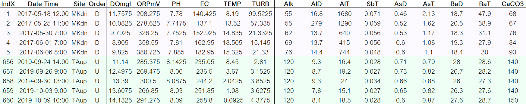
The data include 6 sonde variables and 66 concentration variables (dissolved and total elements, ions, carbonate, organic carbon, nutrient concentrations) (Table 1). The rows are sorted by Site (9 factors), Order (3 factors: up, mid, down), and identified by sampling event: indX (1:660) and Date Time (Year-Month-Day hour:min). Our sampling units are water chemistry samples collected at a site at a specific time. The predictor variables include sonde conductivity (EC) and turbidity (TURB), which are continuous, numeric, and observed. Our response variables are trace element concentrations, which are continuous, numeric, and observed.
Table 1. Head and tail of data table.
|
The benefit of retaining a large suite of sonde and concentration data, rather than reducing the data to a limited suite of trace elements, is that element associations provide more context and are therefore more easily interpreted than individual elements. For example, the interpretation of the chemical availability of lead may vary if it is associated with chlorine and sodium, or calcium carbonate, rather than aluminum. An association with chlorine, sodium, or carbonate may suggest that lead is present in a soluble chemical phase, and therefore may have higher bioavailability to aquatic organisms; an association with aluminum might suggest that the lead in bound in a highly insoluble mineral lattice, and therefore has low potential bioavailability.
Data were collected at 9 sites along four tributary rivers. The data is presented with the following color scheme: Mackay River (purple), Muskeg River (red), Steep Bank River (blue), Tar River (green); upstream (light color), downstream (dark color) (Figure 7). |
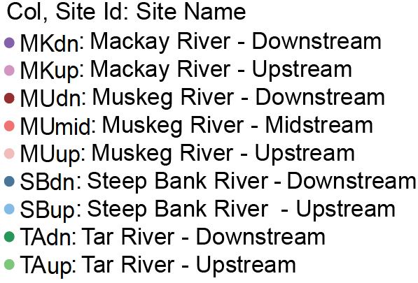
Figure 7. Site color, id, and name guide
|
Cleaning data pre-analysis
With chemical concentration data, measurements below method detection limits are recorded as "NA". Non-sampling events were also recorded as NA. As some multivariate techniques exclude rows (sampling events) which contain NA's; almost the entire dataset was nullified prior to data clean up. Therefore I performed a NA data clean-up.
- First, replicate data were averaged.
- Individual replicate rows and other rows with abundant non-sampling events were removed.
- Non-detects NA's in concentration variables had the value of 0 replace NA if fewer than 25% of sampling events were below detection. Variables which were non-detects in more than 25% of sampling events were excluded from subsequent data analysis (e.g., dissolved lead; ***note, this data still has valuable information, ie. dissolved lead concentrations were low! However, this data cannot not be used in non-robust multivariate analyses).
- For non-concentration variables (e.g. pH, redox-potential, conductivity, water-isotopic composition), NA's were replaced with averages.
Data Normality Scan and Transformation
Principle assumptions of Pearson correlation calculations, Principal Components Analysis, and Discriminate Analysis include data normality and/or homogenous variance among variables. Therefore, histograms (e.g. figure 8, left column) and quantile-quantile plots were used to scan the data for non-normally distributed data.
The majority of concentration and sonde data needed to be transformed. This data non-normality is not surprising in river water concentration data as high-concentration events are relatively rare in natural water quality data, and thus skew the data to the right.
Square-root, logarithmic, and inverse transformations, with the addition of a constant were tested iteratively, to achieve a close-to bell curve data distribution (e.g. figure 8, right column).
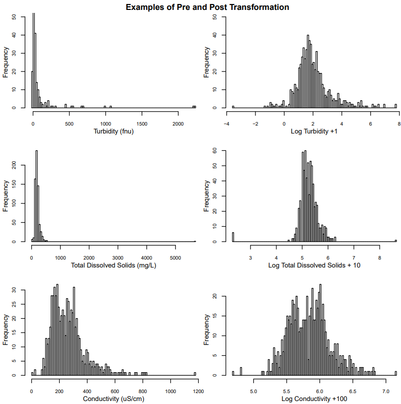
Figure 8. Example histograms of before and after normalization.
Outlier Treatment
Owing to no or limited evidence of sensor malfunction, and due to the non-normal behaviour of water quality data, no outliers were removed. Although rare, extreme or high concentration events are key to understanding system behaviour in hydrology and water quality studies. For example, in small catchments, a single rainstorm can contribute the majority of sediment export for the year; should we not incorporate that anomalous sampling event (high suspended sediment, turbidity, etc) then we may not adequately describe the relation between rainfall and sediment concentration and export. High concentrations of potential contaminants (e.g. lead, mercury, copper, chromium, vanadium) are precisely the events which water quality monitoring efforts aim to observe, and water quality analyses seek to understand and/or model.
Disclaimer: all data and writing within this webpage are for statistics-training purposes only, and were performed on test data.
